3 Nanoscale: molecular motors
In Chapter 2, we presented a modeling framework of the cardiac tissue relying on the additive decomposition of the total stress into a passive and an active contribution. The active stress in the direction of the fiber was written \[ \underline{\underline{\Sigma}}_{{\,a}}= \frac{T_{\text{fib}}}{(1+2\underline{\tau}\cdot\underline{\underline{e}}\cdot\underline{\tau})^{\frac{1}{2}}}\underline{\tau}\otimes\underline{\tau},\quad\text{with } T_{\text{fib}}= \rho_{\text{m}}\tau_{c}+ \nu\dot{e}_{c}, \] where \(\rho_{\text{m}}\) is the number of myosin molecular motors in a layer of thickness \(\ell_{\text{fib}}\) per unit cross-sectional area, \(\tau_{c}\) is the force produced by a single moto and \(\dot{e}_{c}\) is the deformation rate of the half-sarcomere. This chapter summarizes our contribution to the modeling of this force.
The results summarized here are from Caruel, Moireau, and Chapelle, “Stochastic modeling of chemical–mechanical coupling in striated muscles,” 2019; Kimmig and Caruel, “Hierarchical modeling of force generation in cardiac muscle,” 2020; Chaintron, Caruel, and Kimmig, “Modeling actin-myosin interaction: Beyond the huxley–hill framework,” 2023, and Chaintron et al., “A jump-diffusion stochastic formalism for muscle contraction models at multiple timescales,” 2023.
We recall that most of existing heart models use a direct rescaling of the average force generated by an infinitely large population of independent molecular motors, which is equivalent to rescaling the force produced by a single representative motor.
3.1 Background: the myosin molecular motor
3.1.1 Myosin structure

The myosin II protein responsible for muscle contraction consists of two heavy chains containing about 2000 amino-acids each. The two chains are coiled together by their tail regions while their head regions remain independent. A schematic representation one of the chains is shown in figure Figure 3.1 (a).
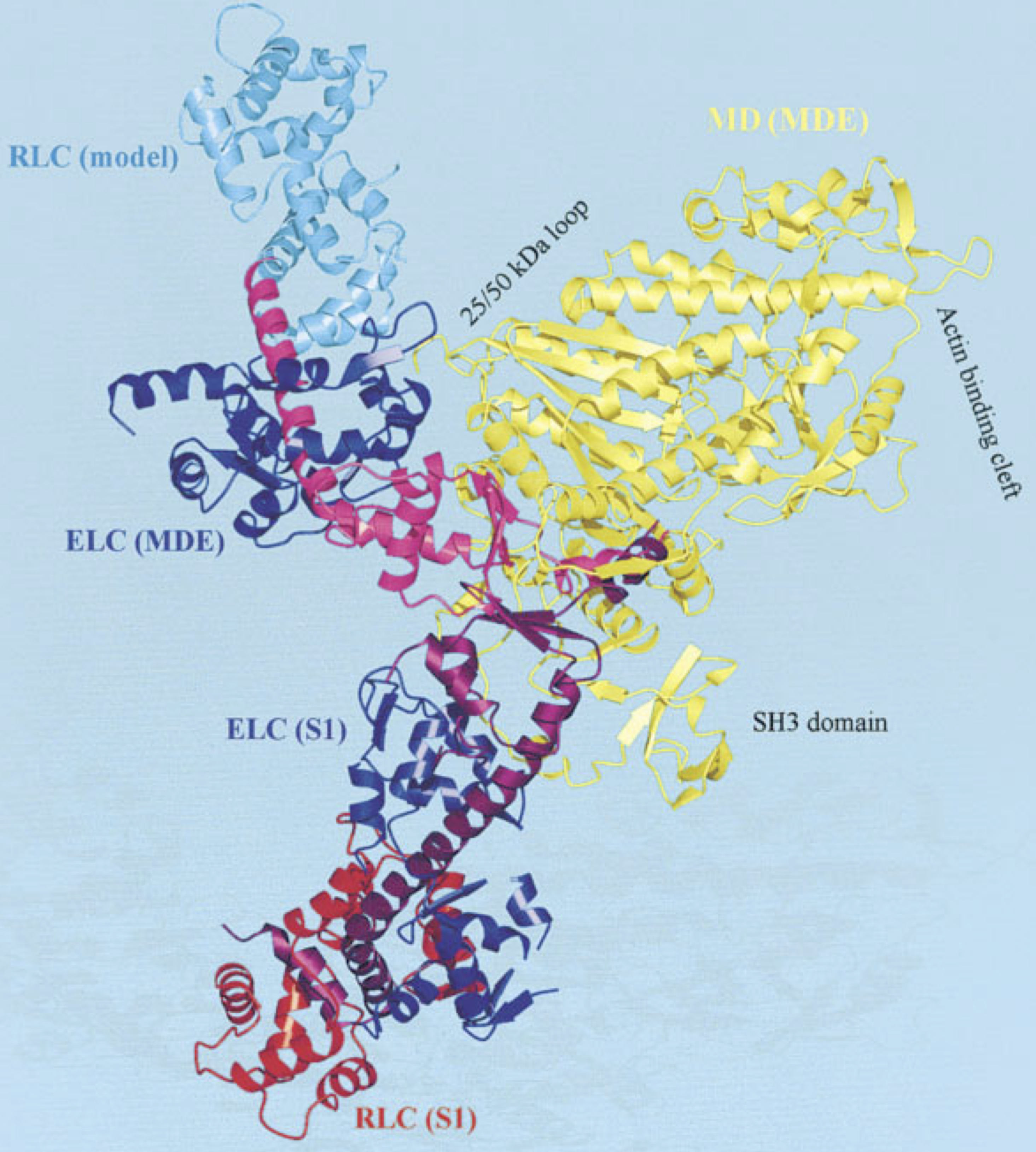
The motor domain is the part of the protein that interacts directly with the actin filament during the contraction. It is connected to a coiled coil called the lever arm, whose christallographic structure has been resolved in the 90s.1 The motor domain itsel is decomposed into several subdomains that surround the active site, where the ATP hydrolysis occurs, see Figure 3.1 (b). A structure of the motor domain of a myosin head (without the lever arm) bound to actin shown in Figure 3.1 (b).
1 Rayment et al., “Structure of the actin-myosin complex and its implications for muscle contraction,” 1993; Dominguez et al., “Crystal Structure of a Vertebrate Smooth Muscle Myosin Motor Domain and Its Complex with the Essential Light Chain: Visualization of the Pre–Power Stroke State,” 1998; Robert-Paganin et al., “Force Generation by Myosin Motors: A Structural Perspective,” 2020.
An important aspect of the force generation mechanism is the ability of the myosin motor domain to undergo a conformational change that gets amplified by the lever arm. In the abence of impairing force (load free condition), the motion of the tip of the lever arm generates a relative displacement of about 10 nm of the myosin filament with respect to the actin filament. This conformational change, called the power stroke (or working stroke) has been characterized from the structural point of view by Dominguez et al.2 A representation of the pre- and post-power stroke structures is shown in Figure 3.2.
3.1.2 Structural aspects of the myosin-actin interaction cycle
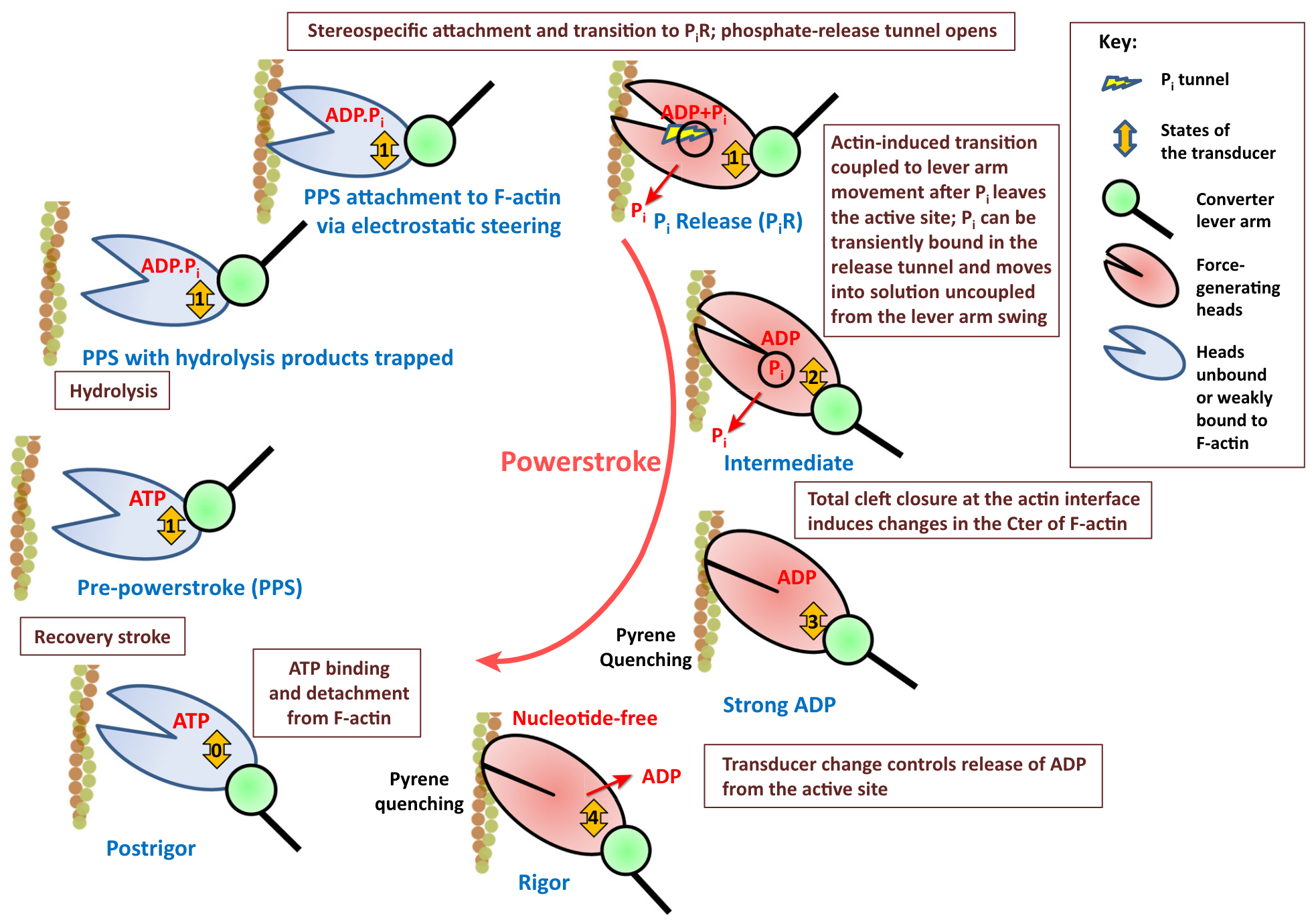
In our Introduction, we presented a simplified version of the Lymn and Taylor cycle, see Figure 1.3. This cycle has been refined since then based on numerous studies that revealed the structures corresponding to various intermediate steps. As an example, the cycle proposed by Houdusse and Sweeney3 is shown in Figure 3.3.
While structural studies undeniably offer valuable insights into the molecular processe of force generation, they do not capture the dynamics of the transitions between the states. However, these structures can serve as initial conditions of Molecular Dynamics (MD) Simulations that can be performed to compute the free energy landscapes between the states as well as and short timescale dynamics.4 Different levels of description are available: all atoms or with different degrees of coarse-graining.5 These costly simulations, even the most coarse-grained ones, can cover timescales up to ~1 μs , which is ineffective to simulate the conformational changes involved in force production which last more than 1 ms .6 Moreover, current MD studies focus on single transitions of the actin-myosin interaction cycle (see Figure 3.3). Simulating the entire ATPase cycle for even a single motor therefore remains a significant challenge.
These simulations however provide valuable information on the effective mechanical properties of the proteins and help to determine the collective variables that can be used to caracterize the different transitions within the cycle. Starting from an all atom dynamics in a space of very high dimension, the strategy is to project this dynamics on lower-dimension manifold parametrized by a set of collective variables to obtain a reduced model.
The highest degree of simplification is when the reduced dynamics becomes a jump process between discrete states, as depicted in Figure 3.3. This description thus views the actin-myosin interaction cycle as a sequence of chemical reactions whose rates determine the dynamics of the system. Most of the currently used molecular motors models are based on this idea, see Section 3.2 for examples.
3.1.3 Single molecule force spectroscopy experiments
Nanomanipulation techniques such as optical tweezers, Atomic Force Microscopy or Scanning probe microscopy, have been developed since the 1990s to study mechanostransduction phenomena of the living cells and in particular force generation by molecular motors.7 They have been particularly successful at determining the functioning of processive molecular motors, i.e. motors that operate individually8 or slow muscles myosins.9 Unlike muscle Myosin II, processive molecular motors stay permanently in contact with their track thanks to their pair of heads actin like coordinated legs. Non processive motors like muscle Myosin II spend only a small fraction of their cycle attached to their track. Studying these short-lived attached configuration requires sub-millisecond resolution of the loading device, which is a technical limitation of single molecule techniques.10
8 Kinesin, Myosin VI etc., see Block, Goldstein, and Schnapp, “Bead movement by single kinesin molecules studied with optical tweezers,” 1990; Svoboda et al., “Direct observation of kinesin stepping by optical trapping interferometry,” 1993; Rock et al., “Myosin VI is a processive motor with a large step size,” 2001; Ménétrey et al., “The structure of the myosin VI motor reveals the mechanism of directionality reversal,” 2005.
10 Finer, Simmons, and Spudich, “Single myosin molecule mechanics: Piconewton forces and nanometre steps,” 1994; Molloy et al., “Single-Molecule Mechanics of Heavy Meromyosin and Si Interacting with Rabbit or Drosophila Actins Using Optical Tweezers,” 1995; Veigel et al., “Load-dependent kinetics of force production by smooth muscle myosin measured with optical tweezers,” 2003.
The development of ultrafast force clamp single molecule spectroscopy over the past decade,11 alows detecting events occuring at timescales comparable to that of the power stroke,12, which partially remove the previous limitations. Before that however, we can mention the work of Veigel et al. on the slower smooth muscle myosin who showed that the myosin detachment rate is load-dependent: it is larger when the molecule is in compression than when in tension.13
A contemporary promising application of single-molecule biophysical experiments is the in-vitro testing of mutated proteins and specific modulators used as treatments of muscular diseases. A recent example is provided by Woody et al.14 where a dual-laser optical trapping setup was used to study the effect of Omecamtiv Mecarbil, a small positive cardiac inotropic agent that increases cardiac performance in acute heart failure situations.15
Since our work is focused on the modeling of non-processive motors, the systematic comparison of the model predictions with single modelule experimental results was not pursued, though it is not excluded for future model calibration procedures.
3.2 Existing models
3.2.1 Chemical-mechanical models
The following is a presentation of the most widely used class of actin-myosin interaction models. While the orginal formulation dates back to the 1950s and 1970s, more recent presentations with additional mathematical and numerical developments can be found in Kimmig, Chapelle, and Moireau, “Thermodynamic properties of muscle contraction models and associated discrete-time principles,” 2019; and Chaintron, Caruel, and Kimmig, “Modeling actin-myosin interaction: Beyond the huxley–hill framework,” 2023. The following paragraphs are adapted from these references.

The typical reprentation of the actin-myosin dynamics is a discrete jump process between states endowed with mechanical degrees of freedom. The first model of this kind was proposed by A.F. Huxley in 1957.16 It has later been formalized and generalized by T.L. Hill and co-workers in 1974.17 Its formulation is illustrated in Figure 3.4.18 The model is parametrized by the distance \(s(t)\) separating the myosin anchor from its nearest binding site. The distance between two consecutive sites is denoted by \(d\). A fundamental hypothesis is that a given head can interact only with the nearest binding site. A myosin head exists in two states: detached or attached to actin, with attachment and detachment events being modeled as a “chemical” jump process with rates that depend on the distance to the nearest binding site \(s\). The Huxley’ 57 model sets the foundation for all subsequent models that use this so-called chemical-mechanical approach.
18 Chaintron, Caruel and Kimmig (“Modeling actin-myosin interaction: Beyond the huxley–hill framework,” 2023) discuss the well-posedness conditions of the Huxley-Hill model and suggest an alternative formulation based on the use of Poisson random measures. We determine conditions that ensure the model’s compatibility with the thermodynamic principles.
The collective variable that lumps the high dimensional space of protein configurations is here the discrete variable \(\alpha_{t}\in\{0,1\}\). This variable characterizes the attachment state of the myosin head, taking the value \(\alpha_{t}=1\) if the head is attached, and the value \(\alpha_{t}=0\) if the head is detached. After attachment, the formed cross-bridge is represented as a spring of elongation \(s(t)\), see Figure 3.4.
The model assumes a large population of independent myosin proteins having their closest attachment sites distributed uniformly in the interval \((-d/2,+d/2)\). Non symetric interval of type \((s_{-},{s_{+}})\) with \(s_{+}-s_{-}=d\) can also be considered. The function \((t,s) \mapsto P_1(t,s)\), represents the fraction of this population that is attached at time \(t\). Similarly, the function \((t,s) \mapsto P_0(t,s) := 1-P_{1}(t,s)\) represents the fraction of this population that is detached at time \(t\).

The stochastic jumps dynamcics associated with \(\alpha_{t}\) involves four transition rates (see Figure 3.5 (a)):
- \(k_{0\rightarrow 1}(s)\) associated with the jump \(0 \rightarrow 1\) (direct attachement);
- \(k^{\mathrm{rev}}_{0\rightarrow 1}(s)\) asociated with the jump \(1 \rightarrow 0\) (reverse attachement);
- \(k_{1\rightarrow 0}(s)\) associated with the jump \(1\rightarrow 0\) (direct detachment);
- \(k^{\mathrm{rev}}_{1\rightarrow 0}(s)\) associated with the jump \(0\rightarrow 1\) (reverse detachment).
These rates can be aggredated by defining \(f(s) = k_{0\rightarrow 1}(s)+k^{\mathrm{rev}}_{1\rightarrow 0}(s)\) and \(g(s) = k_{1\rightarrow 0}(s) + k^{\mathrm{rev}}_{0\rightarrow 1}(s)\). The fraction of attached myosin heads then verifies the following PDE,19 for \(t > 0, \, s \in \left(-\tfrac{d}{2},+\tfrac{d}{2}\right)\) \[ \left\{ \begin{aligned} % & \partial_t P_{1}(t,s) + \xactiveDot(t) \partial_s P_{1}(t,s) =-g(s) P_{1}(t,s) + f(s) \left[1 - P_{1}(t,s)\right], & \partial_t P_{1} + \dot{x}_{c}(t) \partial_s P_{1} =-g(s) P_{1} + f(s) \left[1 - P_{1}\right], \\ & P_{1}(t,\pm d/2) = 0,\; t \geq 0,\\ &P_{1}(0, s) = P^\mathrm{ini}_{1}(s),\; s \in \left[-\tfrac{d}{2},+\tfrac{d}{2}\right], % & P_{0}(s,t) =1 - P_{1}(s,t)&. \end{aligned} \right. \tag{3.1}\] where \(\dot{x}_{c}\) is the relative sliding velocity between the two filaments, see Figure 3.4.
19 This formulation corresponds to the one formulated by Huxley (“Muscle structure and theories of contraction,” 1957).
The tension generated by the attached motors at a given sliding velocity \(\dot{x}_{c}\) is then defined as \[ \tau_{c}(t) := \frac{1}{d} \int_{-d/2}^{+d/2} \partial_s w_1(s) P_{1}(t,s) \mathrm{d}s, \] where \(w_{1}\) is the energy of the protein in the attached state. If the attached protein is viewed as an elastic spring, then \(w_{1}(s) = (\kappa/2)(s-s_{0})^{2}\), where \(\kappa\) is the stiffness and \(s_{0}\) the reference length, see Figure 3.5 (b). This tension is finally rescaled to obtain the macroscopic active stress \(T_{c}\) that appears the macroscopic beharior law, see Section 2.1.3 and Eq. 2.2 in particular.
Overall, the thermodynamic properties of the models are defined by the energy landscapes \(w_{\alpha}\) and by the transition rates. There is no a priori guarantee that for an arbitrary choice of these paramters, the system would be compatible with the principle of thermodynamics. These energetic aspects of the chemical mechanical models have been clarified in the work of Hill.20 In particular, it was shown that the system satisfies the second principle of thermodynamics if for each transition between two states \(A\) and \(B\) of the cycle, the associated transition rates \(K_{A\to B}\) and \(K_{B\to A}\) verify the detailed balance condition \[ \frac{K_{A\to B}}{K_{B\to A}} = \exp\left[-\frac{w_{B}-w_{A}}{k_{\text{B}}T}\right], \] where \(w_{A}\) and \(w_{B}\) are the energies of states \(A\) and \(B\), respectively.
In the case of the two state model illustrated in Figure 3.5 (a), this property reads \[ \begin{aligned} \frac{K_{0\rightarrow 1}(s)}{K^{\mathrm{rev}}_{0\rightarrow 1}(s)} &= \exp\left[-\frac{w_{1}(s) - w_{0}(s)}{k_{\text{B}}T}\right],\\ \frac{K_{1\rightarrow 0}(s)}{K^{\mathrm{rev}}_{1\rightarrow 0}(s)} &= \exp\left[-\frac{(w_{0}(s)-\mu_{T})-w_{1}(s)}{k_{\text{B}}T}\right] \end{aligned} \tag{3.2}\]
Notice that, in the second equation, the energy of the detached state is \(w_{0}-\mu_{T}\) and not \(w_{0}\). The difference is the free energy \(\mu_{T}\) harvested from the hydrolysis of ATP. In isometric condition (\(\dot{x}_{c}=0\)), if \(\mu_{T}=0\), then it can be shown that there is no net flux in the cycle and no force is produced.21
21 Chaintron, Caruel, and Kimmig, “Modeling actin-myosin interaction: Beyond the huxley–hill framework,” 2023; Jülicher and Prost, “Cooperative molecular motors,” 1995.
22 This point is discussed in a general context by Julicher, Ajdari and Prost (“Modeling molecular motors,” 1997), see also Jülicher and Prost, “Cooperative molecular motors,” 1995; Wang and Oster, “Ratchets, power strokes, and molecular motors,” 2002.
A typical cycle is shown by the thick line in Figure 3.5 (b), where we illustrate for each sequence of that cycle, the associated first principle quantity: work (\(\mathcal{W}\)), heat (\(\mathcal{Q}\)) and energy input (\(\\mathcal{E}\)). Having \(\mu_{t}>0\) ensures that, on average the overall free energy decays at each cycle, which maintain non-equilibrium.22
The class of chemical-mechanical models was intensely studied in the late 90’s and up to the late 2010’s, in particular in relation with the development of biomimetic in vitro experiments.23 These works shed light on a variety of dynamical behaviors akin to spontaneous oscillations, emerging particularly when a cluster of motors is coupled to a common elastic substrate.24 Today, the vast majority of existing models pertains to this category and differ from the original Huxley-Hill two state formulation essentially by the number of chemical states involved and by the nature of the spring (linear or nonlinear).25
23 Holzbaur and Goldman, “Coordination of molecular motors: From in vitro assays to intracellular dynamics,” 2010; Pollard, “Evolution of research on cellular motility over five decades,” 2018.
24 We refer to Jülicher and Prost, “Cooperative molecular motors,” 1995; Jülicher, Ajdari, and Prost, “Modeling molecular motors,” 1997; Duke, “Molecular model of muscle contraction,” 1999; Plaçais et al., “Spontaneous Oscillations of a Minimal Actomyosin System under Elastic Loading,” 2009; Guérin et al., “Coordination and collective properties of molecular motors: theory,” 2010 and Guérin, Prost, and Joanny, “Dynamical behavior of molecular motor assemblies in the rigid and crossbridge models,” 2011 for further details.
25 Huxley and Simmons, “Proposed mechanism of force generation in striated muscle,” 1971; Piazzesi and Lombardi, “A cross-bridge model that is able to explain mechanical and energetic properties of shortening muscle,” 1995; Smith and Geeves, “Strain-dependent cross-bridge cycle for muscle. II. Steady-state behavior,” 1995, Smith and Geeves, “Strain-dependent cross-bridge cycle for muscle,” 1995; Duke, “Molecular model of muscle contraction,” 1999; Smith et al., “Towards a Unified Theory of Muscle Contraction. I: Foundations,” 2008; Smith and Mijailovich, “Toward a Unified Theory of Muscle Contraction. II: Predictions with the Mean-Field Approximation,” 2008; Månsson, “Actomyosin-ADP States, Interhead Cooperativity, and the Force-Velocity Relation of Skeletal Muscle,” 2010, Månsson, “Actomyosin based contraction: One mechanokinetic model from single molecules to muscle?” 2016, Månsson, “Hypothesis: Single Actomyosin Properties Account for Ensemble Behavior in Active Muscle Shortening and Isometric Contraction,” 2020; Caremani et al., “Force and number of myosin motors during muscle shortening and the coupling with the release of the ATP hydrolysis products: Chemo-mechanical coupling during muscle shortening,” 2015; Pertici et al., “A myosin II nanomachine mimicking the striated muscle,” 2018.
In summary, the chemical-mechanical models project the high dimensional molecular dynamics on a discrete space of states. The originality of the approach vis a vis a purely chemical system is the association of each state with a mechanical degree of freedom (here denoted as \(s(t)\)). The resuling energy landcape is thereby coupled to the relative position of the two filaments.
3.2.2 Stochastic ratchet models
An alternative to the Huxley-Hill-type models is to consider a less drastic dimensional reduction of the molecular motors’ molecular dynamics, by keeping a description of the “internal motion” of the proteins. Using such approach, the state of the motor is parametrized by a vector of continuous stochastic (collective) variables \(\boldsymbol{X}_{t}\) evolving in a low dimensional space. The dynamics of \(\boldsymbol{X}_{t}\) follows the gradient of an energy landscape wich represent the projection of the all-atom potential on the lower dimension space of collective variables.
A prototype model this kind was proposed by Magnasco.26 The molecular motor is a particle \(X_{t}\in\mathbb{R}\) evolving on a unidimensional periodic energy landscape according to langevin stochastic differential equation
\[ \mathrm{d}X_{t} = -[\phi'(X_{t}) + f(t) + q]\mathrm{d}t + \sqrt{2D}\mathrm{d}B_{t}. \tag{3.3}\]
In Eq. 3.3, \(\phi\) is a non-symetric periodic potential mimicking the interaction with the actin track, \(q\) is the external load, \(D\) is the diffusion coefficient and \(\mathrm{d}B_{t}\) is a brownian motion increment. The term \(f(t)\) represent a so-called colored component of the noise, as opposed to the pure white noise represented by the term \(\mathrm{d}B_{t}\). In the case of Magnasco’s model, it is represented by a deterministic piecewise constant force of the form \(f(t) = A(-1)^{n(t)}\) with \(n(t)=\lfloor 2t/\tau\rfloor\). The average of this force over a period \(\tau\) is equal to 0, implying that \(f\) has no net effect, but combined with the uncorrelated brownian motion and the non-symetric periodic landscape, it can effectively generate a directional motion in the direction opposite to an applied external force. This description is a way to represent the chemical energy input from the ATP hydrolysis as a purely mechanical element.
3.3 Challenges
At the scale of the molecular motor several challenges can be stated.
Not all the crystallographic structures associated with the different steps of the Lymn–Taylor cycle are resolved, and MD simulations only provides very short time dynamics, so one cannot use this technique to simulate the entire interaction cycle. The challenge here is to formulate new methodologies allowing to use the data generated by these simulations to formulate simplified models of the actin-myosin interaction, like for instance the chemical-mechanical models.
A salient feature of the existing chemical-mechanical models is the use of functions to parametrize the transition rates between the states, see \(f\) and \(g\) in Eq. 3.1. These rates are difficult to calibrate in an unequivocal way as they represent a virtually infinite set of parameters. Currently, the data available to constrain their calibration come mostly from experiments dealing with many motors in interaction, different animal species and heterogenous experimental conditions. Other data can be extracted from single molecule experiments. One could also leverage the results of the molecular dynamics simulations on single proteins to complement experiments involving many motors.
The calibration is greatly facilitated by the mean-field assumption mentioned in Section 2.1.3, since it implies a rather direct coupling between the experimental observables and the single motor characterisitcs. This fundamental assumption can be questionned.
3.4 Contributions
3.4.1 The Huxley-Hill formulation revisited
This section is an abstract of the model and results presented in Chaintron, Caruel, and Kimmig, “Modeling actin-myosin interaction: Beyond the huxley–hill framework,” 2023.

Recently, Chaintron, Caruel and Kimmig a published a slightly modified formulation of the Huxley-Hill model,27 see Figure 3.6. In this new formulation, called the h-model, the state of the myosin motor is characterized by three stochastic variables:
- \(X_{t}\), the position of the head with respect to the myosin’s anchor on the thick filament,
- \(h_{t}\), the position of the nearest actin site with respect to \(X_{t}\).
- \(\alpha_{t}\), the attachment state (\(\alpha_{t}=0\) is the motor is detached and \(\alpha_{t}=1\) if it is attached),
The main difference with the original formulation is that the position of the nearest biding \(h_{t}\) site is not anymore defined with respect to the anchor on the thick filament, see Figure 3.4. The two models are linked formally by the relation \(s_{t} = X_{t} + h_{t}\).28 Upon attachment, the variable \(h_{t}\) jumps to 0 so that \(X_{t}=s_{t}\) after attachment.
28 Note that here \(s(t)\) is the distance between the anchor on the myosin filament and the site closest to \(X_t\), which is different from the Huxley-Hill model.
29 mulitisite models in the classical framework can be found in Kimmig, Chapelle, and Moireau, “Thermodynamic properties of muscle contraction models and associated discrete-time principles,” 2019 and Månsson, “Comparing models with one versus multiple myosin-binding sites per actin target zone: The power of simplicity,” 2019.
The consequence of this seemingly innocent change is that the myosin head can now attach to any site on the real axis without having to resolve to an explicitly multi-site formulation.29 Using a multi-site model comes at the price of having to define four rates per additional site. While we still enforce the myosin head to interact with only one site at a time, it can now be any site with only four rates to calibrate.
Chaintron Caruel and Kimmig30 formulate this new approach using the concept of Poisson random measures,31 and establish the conditions of its well posedness. We adapt the detailed balance condition (3.2) and show the ensuing model’s compatibility with the second principle. We then propose a reduction strategy that allows to adiabatically eliminate the variable \(h_t\). The resulting reduced model has only two degrees of freedom, namely \(s\) and \(\alpha\), like the Huxley-Hill model. The associated PDE formulation is analog to Eq. 3.1 with a correction term. This shows that by extrapolation, more complex chemical-mechanical models (i.e. with more states) could be reformulated using this new framewotk. The paper also provide numerical illustrations of the h-model and of its reduced version.
31 The interested reader can find a short pedagogical introduction to the concept of Poisson Random measured in section 2.2 of Chaintron, Caruel, and Kimmig, “Modeling actin-myosin interaction: Beyond the huxley–hill framework,” 2023.
3.4.2 Continuous model of the working stroke
This work was initiated by Marcucci and Truskinovsky (“Mechanics of the power stroke in myosin II,” 2010) and continued during M. Caruel’s PhD. Details about the model can be found in the following references: Caruel, Allain, and Truskinovsky, “Muscle as a Metamaterial Operating Near a Critical Point,” 2013 and Caruel and Truskinovsky, “Physics of muscle contraction,” 2018. Note also that the latter reference is already a review of several papers by Caruel and Truskinovsky.
The working stroke is the force-generating step of the actin-myosin interaction cycle, see Figure 1.3. It corresponds to a conformational change of the protein executed while it is attached to the actin filament. This transition can be interpreted as the swift relaxation towards thermal equilibrium of the internal degrees of freedom characterizing the conformation of the myosin protein, with an associated timescale of a few milliseconds. This timescale is short compared to the time to complete the Lymnn-Taylor cycle (about 30 ms), which suggests that the power stroke is a purely mechanical phenomenon.32
32 Huxley and Simmons, “Proposed mechanism of force generation in striated muscle,” 1971; Marcucci and Truskinovsky, “Mechanics of the power stroke in myosin II,” 2010; Caruel and Truskinovsky, “Physics of muscle contraction,” 2018.
33 Huxley and Simmons, “Proposed mechanism of force generation in striated muscle,” 1971; Smith et al., “Towards a Unified Theory of Muscle Contraction. I: Foundations,” 2008; Caremani et al., “Force and number of myosin motors during muscle shortening and the coupling with the release of the ATP hydrolysis products: Chemo-mechanical coupling during muscle shortening,” 2015; Månsson, “Actomyosin based contraction: One mechanokinetic model from single molecules to muscle?” 2016.
In the classical framework of chemical-mechanical models presented in Section 3.2.1, the power stroke is viewed as a sequence of three or more chemical transitions.33 While the molecular structures of the pre- and post-power-stroke conformations have been clearly identified,34 additional states are not yet associated with stable structure.
Furthermore, since the motion of the lever arm is by essence constrained by the relative motion of the myosin and actin filaments, which is not a discrete process, it seems natural to view the power-stroke as a continuous process, an idea that was originally coined by Eisenberg and Hill.35 Finally, from a mathematical point of view, studying the low temperature limit of a continuous power-stroke model could help to justify the discrete approach.

Based on the experimental observation, first made by Huxley and Simmons36, that the power stroke operates at fast timescales, Marcucci and Truskinovsky developed a model of the working stroke, where the conformational change is represented as a one-dimensional Langevin process in a double-well potential instead of a jump process, see Figure 3.7. This model can be considered as a regularized version of the original chemo-mechanical representation of the working stroke proposed by Huxley and Simmons.
The model was introduced to model the collective response of groups of connected molecular motors to rapid load changes. This topic will be discussed in details in Chapter 4. We now present how this continuous model of the power stroke can be coupled to a more classical “chemical” representation of the attachment-detachment process, to result in a hybrid jump-diffusion model actin-myosin interaction model.
3.4.3 Jump-diffusion model of the Lymn–Taylor cycle
The formulation of the model and its first validation are from Caruel, Moireau, and Chapelle, “Stochastic modeling of chemical–mechanical coupling in striated muscles,” 2019. The model was further refined and calibrated to reproduce cardiac muscle data during the PhD of F. Kimmig in Kimmig and Caruel, “Hierarchical modeling of force generation in cardiac muscle,” 2020. Recently the formulation of the model was significantly improved, with the contribution of L. P. Chaintron, to streghthen its mathematical well-posedness and assess its compatibility with the thermodynamic principles in Chaintron et al., “A jump-diffusion stochastic formalism for muscle contraction models at multiple timescales,” 2023.

To extend the Marcucci and Truskinovsky model37 of the power stroke, and describe the whole Lymn–Taylor cycle, Caruel, Moireau and Chapelle proposed a jump-diffusion hybrid model,38 illustrated in Figure 3.8 (a). The state of the myosin motor is parametrized by the following stochastic variables
- \(X_{t}\), the position of the myosin head with respect to its fixed location on the myosin filament,
- \(Y_{t}\), the conformation of the head (power stroke),
- \(\alpha_{t}\), the state of attachement (equal to 0 when the motor is detached and equal to 1 when the motor is attached).
As in the classical Huxley-Hill model, the myosin head can attach only to the nearest actin site, located at a distance \(s\) from the myosin anchor in the thick filament. When an attachment event (\(\alpha=0\to\alpha=1\)) occurs, the head position jumps to the value \(X_{t} = s(t)\).
The stochastic jump dynamics is formulated by Chaintron et al. using the concept of Poisson random measures, which allows to write the stochastic differential equation describing the dynamics of the discrete variable \(\alpha_{t}\).39 The jump process involves four transition rates
- \(K_{0\rightarrow 1}(x,y,s)\) associated with the jump \(0 \rightarrow 1\) (direct attachment);
- \(K^{\mathrm{rev}}_{0\rightarrow 1}(x,y,s)\) associated with the jump \(1 \rightarrow 0\) (reverse attachment);
- \(K_{1\rightarrow 0}(x,y,s)\) associated with the jump \(1\rightarrow 0\) (direct detachment);
- \(K^{\mathrm{rev}}_{1\rightarrow 0}(x,y,s)\) associated with the jump \(0\rightarrow 1\) (reverse detachment).
The conformation variable \(Y_{t}\) and the detached head position \(X_{t}\) both follow langevin dynamics. As in the classical Huxley-Hill formulation, the internal energy of the myosin motor depends on the attachment state. A typical actin-myosin interaction cycle is illustrated in Figure 3.8 (b). Within this theoretical formalism, the complete jump-diffusion stochastic differential system can be written as
\[ \left\{ \begin{aligned} &\begin{split}\mathrm{d}\alpha_t &= \mathbb{1}_{\alpha_{t^-} = 0} \left[ \int_{\mathbb{R}_+} \mathbb{1}_{ z \leq K_{0\rightarrow 1}( X_{t^-} , Y_{t}, s(t) )} N_{0\rightarrow 1}( \mathrm{d}t , \mathrm{d}z ) +\int_{\mathbb{R}_+} \mathbb{1}_{z \leq K^{\mathrm{rev}}_{1\rightarrow 0}( X_{t^-} , Y_{t}, s(t) ) } N^{\mathrm{rev}}_{1\rightarrow 0}( \mathrm{d}t , \mathrm{d}z ) \right]\\ & \phantom{ab} - \mathbb{1}_{\alpha_{t^-} = 1} \left[ \int_{-d/2}^{+d/2} \int_{\mathbb{R}_+} \mathbb{1}_{z \leq K_{1\rightarrow 0}( x, Y_{t}, s(t) )} N_{1\rightarrow 0}( \mathrm{d}t , \mathrm{d}x , \mathrm{d}z) \right.\\ & \hspace{2cm}+ \left.\int_{-d/2}^{+d/2} \int_{\mathbb{R}_+} \mathbb{1}_{z \leq K^{\mathrm{rev}}_{0\rightarrow 1}( x, Y_{t}, s(t) )} N^{\mathrm{rev}}_{1\rightarrow 0}( \mathrm{d}t , \mathrm{d}x , \mathrm{d}z ) \right], \\ \end{split}\\ &\begin{split} \mathrm{d}X_t &= \mathbb{1}_{\alpha_{t^-} = 0} \left[ -\eta_x^{-1} \partial_x w_{0} ( X_t , Y_t ) \mathrm{d}t + \sqrt{2 \eta^{-1}_x k_B T}\, \mathrm{d}B^x_t \right] + \mathbb{1}_{\alpha_{t^-} = 1} \dot{x}_{c}(t) \mathrm{d}t \\ & \phantom{ab}+ \mathbb{1}_{\alpha_{t^-} = 0} \left[ \int_{\mathbb{R}_+} ( s({t}) - X_{t^-} ) \mathbb{1}_{z \leq K_{0\rightarrow 1}( X_{t^-} , Y_{t}, s(t) )} N_{0\rightarrow 1}( \mathrm{d}t , \mathrm{d}z ) \right.\\ & \hspace{2cm}+ \left.\int_{\mathbb{R}_+} ( s(t) - X_{t^-} ) \mathbb{1}_{z \leq K^{\mathrm{rev}}_{1\rightarrow 0}( X_{t^-} , Y_{t}, s(t) ) } N^{\mathrm{rev}}_{1\rightarrow 0}( \mathrm{d}t , \mathrm{d}z ) \right] \\ & \phantom{ab}+ \mathbb{1}_{\alpha_{t^-} = 1} \left[ \int_{-d/2}^{+d/2} \int_{\mathbb{R}_+} ( x - s(t) ) \mathbb{1}_{ z \leq K_{1\rightarrow 0}(x, Y_{t}, s(t) )} N_{1\rightarrow 0}( \mathrm{d}t , \mathrm{d}x , \mathrm{d}z) \right. \\ & \hspace{2cm}+ \left.\int_{-d/2}^{+d/2} \int_{\mathbb{R}_+} ( x - X_{t^-} ) \mathbb{1}_{z \leq K^{\mathrm{rev}}_{0\rightarrow 1}(x, Y_{t}, s(t) )} N^{\mathrm{rev}}_{0\rightarrow 1}( \mathrm{d}t , \mathrm{d}x , \mathrm{d}z) \right], \\ \end{split}\\ &\mathrm{d}Y_t = -\eta_y^{-1} \partial_y w_{\alpha_t} ( X_t , Y_t ) \mathrm{d}t + \sqrt{2 \eta^{-1}_y k_B T}\, \mathrm{d}B^y_t, % \end{split} \end{aligned} \right. \]
where \(\eta_{x,y}\) are drag coefficients, and \((B_{t}^{x})_{t\geq 0}\) and \((B_{t}^{y})_{t\geq 0}\) are independent Brownian motions.40 Notice that, in the second equation, the motion of \(X_{t}\) is determinitic when the head is attached, like in the two state model presented in Section 3.2.1.
40 The meaning of the integrals of the form \(\int_{0}^{t}\int_{\mathbb{R}_{+}}F(t,z)N(\mathrm{d}t,\mathrm{d}z)\) is explained in more details with extra references and numerical implementation in Section 2.2 and 4.1 of Chaintron et al., “A jump-diffusion stochastic formalism for muscle contraction models at multiple timescales,” 2023.
The peculiarity of this model lays in the assymetry between the attachment and the detachment jumps, which results from the different system’s dimensionality in the attached and detached states. When the motor is detached, it evolves in a two dimenional space \((X_{t},Y_{t})\), while when it is attached, \(X_{t}=s(t)\) so the dynamics besomes one dimensional. Hence, when an attachment jump occurs from a random configuration \((X_{t},Y_{t})\), the dynamics is projected on a one dimensional space, parametrized by \(s(t)\). Hence, the value of \(X_t\) after the jump is fully determined by the position of the site.
The situation is different with the detachment, since there is no a priori value prescribed for \(X_{t}\) after the jump. This discrete-to-continuous detachment jump must then select a random location \(x\) for the detached myosin head. The probability law that chooses this new location has to be defined carefully to preserve the thermodynamic compatibility.
This problem was solved41 by considering the total jumps \((0,x,y,s)\to (1,s,y,s)\to(0,x,y,s)\) and writing the detailed balance conditions \[ \left\{ \begin{aligned} K_{0\rightarrow 1}(x,y,s) &= h_x \exp \biggl[ -\frac{w_1(s,y) - w_0(x,y) }{k_B T} \biggr] K^{\mathrm{rev}}_{0\rightarrow 1}(x,y,s),\\ K_{1\rightarrow 0}(x,y,s) &= h^{-1}_x \exp \biggl[ -\frac{(w_0(x,y) - \mu_T) - w_1(s,y) }{k_B T} \biggr] K^{\mathrm{rev}}_{1\rightarrow 0}(x,y,s), \end{aligned} \right. \tag{3.4}\] where \(h_{x}\) is a characteristic length for \(x\), taken equal to the characteristic length of the power stroke. Provided Eq. 3.4, only two rates have to be calibrated. From the rate \(K_{1\rightarrow 0}\) one can define the global detachment rate, describing the frequency of the detachment, considering all detached positions \(x\) that can be reached from an attached configuration \((1,s,y,s)\) \[ k_{1\rightarrow 0}(y,s) = \int_{-d/2}^{d/2}K_{1\rightarrow 0}(x,y,s)\mathrm{d}x, \] A similar rate \(k^{\mathrm{rev}}_{0\rightarrow 1}\) can be defined for the reverse attachment jump rate \(K^{\mathrm{rev}}_{0\rightarrow 1}\). The rates \(k_{1\rightarrow 0}\) and \(k^{\mathrm{rev}}_{0\rightarrow 1}\) are analog to the rates presented in Section 3.2.1. In the numerical implementation of the jump-diffusion process, the global rates \(k_{1\rightarrow 0}\) and \(k^{\mathrm{rev}}_{0\rightarrow 1}\) are used to termine the time between consecutive jumps. When a detachment jump occurs, the jump amplitude is drawn from the probability law \(k_{1\rightarrow 0}(y,s)^{-1}K_{1\rightarrow 0}(x,y,s)\mathrm{d}x\) (or \(k^{\mathrm{rev}}_{0\rightarrow 1}(y,s)^{-1}K^{\mathrm{rev}}_{0\rightarrow 1}(x,y,s)\mathrm{d}x\))42.
41 Chaintron et al. “A jump-diffusion stochastic formalism for muscle contraction models at multiple timescales,” 2023
42 see Section 4.1 and 4.2 of Chaintron et al., “A jump-diffusion stochastic formalism for muscle contraction models at multiple timescales,” 2023 for the details

The model developed by Chaintron et al.43 has been calibrated to reproduce data obtained on rat trabeculae in various experimental studies. In Figure 3.9, we show an extract of the results illustrating the Hill force-velocity curve. The model faithfully reproduces the fast transient response to rapid load changes44, and can be used to predict the thermodynamic efficiency of the contraction.
43 “A jump-diffusion stochastic formalism for muscle contraction models at multiple timescales,” 2023.
44 see figure 6 and 7 of Chaintron et al., “A jump-diffusion stochastic formalism for muscle contraction models at multiple timescales,” 2023. For the details about the calibration procedure, we refer to Kimmig and Caruel, “Hierarchical modeling of force generation in cardiac muscle,” 2020 and Chaintron et al., “A jump-diffusion stochastic formalism for muscle contraction models at multiple timescales,” 2023
3.4.4 Mean field approximation
We here recall that the active force produced by the motors, \(\tau_{c}\) enters the macroscopic balance law throught the active stress (see Figure 2.2) \[ \underline{\underline{\Sigma}}_{{\,a}}= \frac{T_c+ \nu \dot{e}_{c}}{(1+2\underline{\tau}\cdot\underline{\underline{e}}\cdot\underline{\tau})^{\frac{1}{2}}}\underline{\tau}\otimes\underline{\tau},\quad\text{with } T_c= \rho_{\text{m}}\tau_{c},\text{ and } \dot{e}_{c}= \dot{x}_{c}/\ell_{\text{fib}}, \tag{3.5}\] where \(\dot{x}_{c}\) is the relative sliding velocity between the filament. In the jump diffusion model presented in the previous section, if one considers a cluster of \(N\) motors, the force \(\tau_{c}\) reads \[ \tau_{c}= \kappa\frac{1}{N}\sum_{i=1}^{N} \alpha_{t}^i(X_t^{i} + Y_t^i). \tag{3.6}\] This force, produced by the attached motors, is linked to the sliding velocity \(\dot{x}_{c}\) by the macroscopic balance law (3.5), which effectively creates a mechanical coupling between the force generating units. Notice that this coupling has no effect on the detached motors.
Most of the existing models are based on the assumption that, in the regime of a large number \(N\) of motors, the total macroscopic force \(T_c\) defined in Eq. 3.6, which in principle is random and depends on the state of the (attached) motors, can in fact be considered deterministic and given by \[ T_c= \rho\kappa\,\mathbb{E}[\alpha_{t}(X_t + Y_t)], \] where the expectation is taken by averaging over the statistical distribution of a single motor. This assumption reduces the study of a system of \(N\) interacting motors to that of a single one interacting with a surrounding mean-field, which is generally given by the solution of a nonlinear partial differential equation like Eq. 3.1 in the case of the Huxley-Hill model. In the case of the jump-diffusion model presented above, the computation of the active force necessitates the simulation of a large number of stochastic realizations of the processes \(\alpha_{t}\), \(X_{t}\) and \(Y_{t}\). In a finite element simulation framework this operation has to be performed at each material point, which comes at a high computational cost. This limitation has been addressed by Kimmig and Caruel,45 who derived several reduced version of the jump-diffusion model.
3.4.5 Reduced models
The reduced models presented in this section are from Kimmig and Caruel, “Hierarchical modeling of force generation in cardiac muscle,” 2020 with preliminary results from Bestel, Clément, and Sorine, “A Biomechanical Model of Muscle Contraction,” 2001; Chapelle et al., “An energy-preserving muscle tissue model: Formulation and compatible discretizations,” 2012 and Caruel et al., “Dimensional reductions of a cardiac model for effective validation and calibration,” 2014.

The first reduced model is obtained by eliminating the dynamics of the conformational variables \(X_{t}\) and \(Y_{t}\), see Figure 3.10. This elimination is justified by the separation of timescales between the power stroke conformational change and the attachment-detachment process. The approximation consists in considering that \(X_{t}\) and \(Y_{t}\) quickly relax towards equilibrium, and are therefore distributed according to the classical Boltzmann density at fixed \(s(t)\). The ensuing model has only two states see 3.10 and becomes analogous to the classical Huxley-Hill model (see Eq. 3.1), with the peculiarity that the free energies characterizing the two states and the transition rates are derived from a more refined model.
The system can be further simplified by considering the moments of the distribution \(P_{1}(s,t)\) of heads in the attached states:46 \[ M_{p} = \frac{1}{d}\int_{s_{-}}^{s_{+}}s^{p}P_{1}(s,t)\mathrm{d}s. \] Using the conservation equation (3.1) we can write the following unclosed system of ordinary differential equations (ODE) \[ \dot{M}_{p}(t) = p\dot{x}_{c}M_{p-1}(t) + f_{p} - \frac{1}{d}\int_{s_{-}}^{s_{+}}(f(s) + g(s))s^{p}P_{1}(s,t)\mathrm{d}s, \] with \(f_{p} = \frac{1}{d}\int_{s_{-}}^{s_{+}}s^{p}f(s)\mathrm{d}s\). This system of ODEs is equivalement to solving Eqs. 3.1, but specific closure relations can limit its size. For instance, if we assume that (i) the sum \(f(s)+g(s)\) is independent of \(s\)47 and that the energy of the attached state is quadratic (as in the classical Huxley Hill model), the moment equations reduce to \[ \left\{ \begin{aligned} \dot{K}_{c}(t) &= -(f+g)K_{c}(t) + f_{0}K_{\infty},\\ \dot{T}_{c}(t) & = -(f+g)T_{c}(t) + \dot{x}_{c}K_{c}(t) + (s_{0}f_{0}+f_{1})K_{\infty}, \end{aligned} \right. \] where \(K_{c} = \rho\kappa M_{0}\), \(K_{\infty} = \rho\kappa\), and \(T_{c} = \rho\kappa(s_{0}M_0+M_{1})\) depend on the 0th and 1st order moments. In the steady state regime, the prediced force-velocity relation is linear: \[ T_{c}^{\infty} = \frac{f_{0}K_{\infty}}{(f+g)^{2}}\dot{x}_{c}+ \frac{s_{0}f_{0}+f_{1}}{f+g}K_{\infty}, \] which is incompatible with observations, see Figure 3.9.
46 We here consider a single site model, see Kimmig and Caruel, “Hierarchical modeling of force generation in cardiac muscle,” 2020 for the multi-site formulation.
However, Kimmig and Caruel48 showed that, despite its simplicity, a linear force velocity relation satifactorily reproduces the mechanical output of a muscle fiber in a regime compatible with the deformation rates observed in a contacting heart.
3.5 Ongoing work
3.5.1 Molecular dynamics study of the Lymn–Taylor cycle
This topic is the motivation of R. Manevy’s the PhD thesis at MSME. It is done in collaboration with A. Houdusse from Institut Curie. This work has been presented in several conferences and workshop: Caruel et al., “Umbrella Sampling for the estimation of the free energy barrier of Pi release in Myosin,” 2022; Manevy et al., “Étude mécanique d’une protéine du muscle,” 2021, Manevy et al., “Identification of Free Energy Barriers Associated With Transition In Myosin cycle Using Umbrella Sampling,” 2021. A journal article is in preparation.
The objective of this work is to close the gap between structural mechanisms of the molecular motors functioning inferred from crystallographic data and more coarse theoretical models. The strategy is to project the high-dimension dynamics of the molecular system onto a low dimension manifold, enabling physiological timescale simulations based on Stochastic Differential Equations alike the ones presented in section Section 3.4.3.
For instance, the parameters characterizing energy landscape that is used to describe the power stroke are usually calibrated using data from fast load change experiments performed on muscle fiber.49 One could also compute this energy landscape from molecular dynamics simulations.
49 Marcucci and Truskinovsky, “Mechanics of the power stroke in myosin II,” 2010; Caruel, Moireau, and Chapelle, “Stochastic modeling of chemical–mechanical coupling in striated muscles,” 2019; Kimmig and Caruel, “Hierarchical modeling of force generation in cardiac muscle,” 2020.
50 see Llinas et al., “How Actin Initiates the Motor Activity of Myosin,” 2015, for a review on the topic
In the PhD work of R. Manevy, we studied the step of the actin-myosin interaction cycle where the inorganic phosphate (Pi), a product of the ATP hydrolysis, is released from the active site. The interplay between this escape from the active site and the power stroke conformational change is a subject of debate: is the release occuring before or after the working stroke, or can they occur simultaneously?50
To test different escape pathways and their associated energetic costs, we performed Umbrella Sampling simulations starting with two crystallographic structures and several local configuraiton of the Pi within the active site, see Figure 3.11.
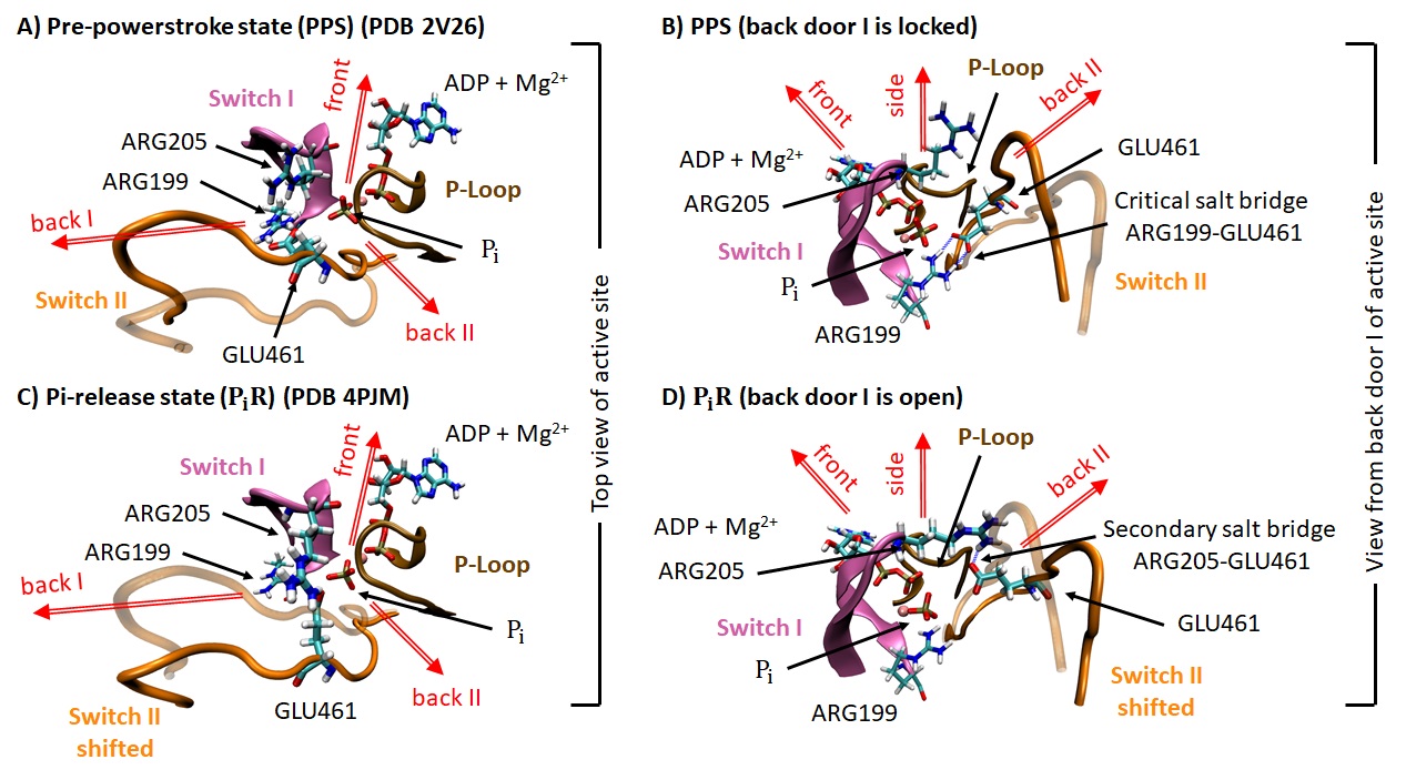
The constraint is the distance between the Pi and the magnesium ion associated with ADP in the active site. By increasing this distance in a step-by-step manner, we force the inorganic phosphate out of the active site. The potential of mean force characterizing this process can be reconstructed, giving an estimate of the energy barrier associaed with the escape pathway taken by the Pi. An example of the escape process is illustrated in Figure 3.12. Only the strutures surrounding the active site are shown for clarity.
We found that the initial condition of the simulation, and in particular the orientation of the Pi within the active site, greatly affects the escape pathway and the associated potential of mean force. The statistical validation of these observations are work in progress.
3.5.2 Purely mechanical model of the actin-myosin interaction
This work is a follow-up of our collaboration with L. Truskinovsky and R. Sheshka. Preliminary work can be found in Sheshka and Truskinovsky, “Power-stroke-driven actomyosin contractility.” 2014 and section 4.2 of Caruel and Truskinovsky, “Physics of muscle contraction,” 2018.
In Section 3.4.3, we presented a hybrid chemical-mechanical framework of the actin-myosin interaction. As mentioned in Section 3.2, there exists a category of models where the dynamics of the molecular motor is represented as a Langevin-type drift-diffusion process with a colored noise. The prototypical example of this class of models was proposed by Magnasco, see Eq. 3.3.

In Figure 3.13 we present an extension of Magnasco’s model that includes the power stroke mechanism. The molecular motor is parametrized by the position of the head \(X_{t}\) and the position of the tip of the lever arm \(Y_{t}\). Both variables are endowed with Langevin stochastic dynamics. The associated potential includes.
- the energy landscape \(\Phi\) which represents the interaction between the tip of the head and the actin track (a),
- the bistable potential \(u_{\text{ss}}\) representing the power stroke conformational change energetics (b).
As in Magnasco’s model, the colored component of the noise is a piecewise constant periodic force \(f\) that operates on the variable \(Y_{t}-X_{t}\), i.e. on the power stroke, see Figure 3.13 (c). The action of this periodic force on the power stroke is the mechanical representation of the energy input provided by ATP hydrolysis. The directionality of the motion can be achieved either by making the actin interaction potential \(\Phi\) non symetric or by introducing a control mechanism \(d(Y_{t}-X_{t})\in[0,1]\), that mimicks the coupling between mechanics and biochemistry in the Lymn–Taylor cycle. The potential of the system can then be written as \[ G(x,y,d,t) = d\Phi(x) + u_{\text{ss}}(y-x) + f(t)(y-x) - f_{\text{ext}}y, \tag{3.7}\] where \(f_{\text{ext}}\) is the external force. The dynamics of the system is then written as \[ \left\{ \begin{aligned} \mathrm{d}X_{t} &= -\partial_{x}G(X_{t},Y_{t},d,t)\mathrm{d}t + \sqrt{2D}\mathrm{d}B_{t}^{x},\\ \mathrm{d}Y_{t} &= -\partial_{y}G(X_{t},Y_{t},d,t)\mathrm{d}t + \sqrt{2D}\mathrm{d}B_{t}^{y}. \end{aligned} \right. \] In Eq. 3.7, the coupling \(d\) characterizes the strength of the attachment. When \(d=1\), the actin potential affects on the evolution of \(X_{t}\), effectively modeling the attachment. When \(d=0\), the interaction with actin is turned “off”, which represents the detached state.
Considering the dependence of \(d\) on the power stroke conformation \(Y_{t} - X_{t}\) shown in Figure 3.13 (f), the multiplicative combination of \(d\) and \(\Phi\) effectivety mimicks the loss of affinity of the myosin head for actin as the power stroke conformational change happens. At the begining of the power stroke \(Y_{t}-X_{t}\approx -a/2\), so \(d=1\). Therefore, the gradient actin potential participates in driving the position \(X_{t}\). After the completion of the power stroke \(Y_{t}-X_{t}\approx a/2\), so \(d=0\). Therefore, the contribution of the actin potential to the motion of the head vanishes, mimicking a detached state.
An interesting characteristic of this family of model involving a control parameter is that directionality can be achieved even if all the potentials are symetric, like shown in Figure 3.13. More refined version of the coupling \(d\) can incorporate memory effect which can, according to the preliminary results of Sheshka and Truskinovsky,51 augments the mechanical performance of the motor, see Figure 3.14.

3.6 Other project: nano diffusion in the bone tissue
The biomechanics team of the MSME laboratory actively work on the mechanics of bone remodeling at various scales. Biochemical signaling for bone remodeling involves ionic diffusion within nanopores that connect bone cells to each other. We used molecular dynamics tools to simulate confined diffusion at the nanoscale and determine the physical parameters (diffusion tensor, viscosities, etc.) associated with the flow in the nanopores. This work enabled the determination of relevant parameters for a multiscale model of bone remodeling and also contributed to the understanding of the molecular mechanism of intercellular signaling within the bone tissue.52
3.7 Remaining challenges and future work
3.7.1 Beyong the mean-field hypothesis
- In the applied mathematics and statistical physics literature, the fact that the mean-field model summarized in Section 3.4.4 actually describes the large \(N\) limit of the original model is called the propagation of chaos phenomenon.53 It finds its roots in the kinetic theory of gas dynamics but has found applications in a wide range of domains, including biology, game theory or deep learning. The quantitative study of this phenomenon, and in particular of the regime in which it occurs, is an active field of research at the interface between probability theory, partial differential equations and statistical physics.54
A natural follow-up of the work on the jump-diffusion model presented in Section 3.4.3 is thus to reconsider the mean-field hypothesis and model a finite size cluster of interacting molecular motors. This line of research was started by Caruel, Allain and Truskinovsky (“Muscle as a Metamaterial Operating Near a Critical Point,” 2013) and will be presented in more detailed in the next c]hapter.
The question raised is the representation of the mode of interaction between the motors. One approach consists in considering short range elastic interactions between motors that are attached on the same actin filament. In this way, next-to-nearest neighbors cooperative mechanisms can emerge and propagate inside the contractile unit. This extension of a finite size system will also be useful to compare the model predictions with experimental measurements performed on synthetic nanomachines mimicking the muscle contractile units.55
3.7.2 Molecular dynamics simulations
The potential next steps of R. Manevy’s thesis discussed in Section 3.5.1 are to extend the current study to the other steps of the Lymn–Taylor cycle and to strengthen of the methodology used for determining the adequate collective variables characterizing the conformational changes.
This work heavily relies on the availability of crystallographic structures serving as initial (or final) condition for these simulations. These structures are not always available in the protein databank, which limits the applicability of a model calibration approach based solely on molecular dynamcis simulations. In particular, it still seems difficult to simulate detachment or attachments events using these techniques before establishing the structural basis of the affinity of myosin for actin.
Choosing appropriate collective variables to describe the motion of the protein during a conformational change is not easy. The energy landscape characterizing the protein is high-dimensional and very rugged so that (i) the collective variables found numerically may not be the most representative (i.e. the fastest) and (ii) the sampling of the effective free energy landscape ineffective. Our future work will involve exploration of various sampling methods and potential use of AI based techniques.56